Quick and Easy Standalone Webmaps Using GeoPandas
NNIP Idea Showcase
June 20, 2024
Adam Porr
Research & Data Officer
Mid-Ohio Regional Planning Commission
Abstract
Lots of great third-party platforms are available which allow users to create interactive webmaps to present spatial data including ArcGIS Online, Google Maps, and Mapbox. These services are appropriate for many use cases, however some situations may warrant a standalone webmap that is not reliant on a third party platform. Such situations might include budget constraints, special access control requirements, special user interface requirements, the desire to package the content or implement version control, or the need to access the webmap in an environment without internet access. In such cases, it is possible to develop a standalone webmap from scratch using frameworks such as Leaflet or OpenLayers, however this can be time consuming, and it requires knowledge of Javascript programming and web server administration. Luckily, the excellent GeoPandas package for Python provides a means of producing basic webmaps that is more accessible to Python programmers and avoids much of the complexity and tedium of building the webmap from scratch. This presentation demonstrates how to automatically produce an interactive standalone webmap using vehicle access data from U.S. Census API and bike infrastructure data from an ArcGIS REST API using GeoPandas. The workflow is implemented using Jupyter to allow for convenient prototyping of the webmap prior to production. The presentation also covers how to make the webmap accessible to the public using GitHub Pages.
Attendee familiarity with Python, Jupyter, and GitHub is helpful but not required.
Agenda
- Motivation
- Process overview and prerequisites
- Data preparation (skipped in presentation)
- Demo of webmap creation and export
- Demo of webmap publishing using GitHub Pages
How to access the content from this presentation
All of the content presented today is publicly available in GitHub:
https://github.com/aporr/easy-webmaps-with-geopandas
The webmap is available directly from the following URL:
https://aporr.github.io/easy-webmaps-with-geopandas/webmap.html
GeoPandas can make simple webmaps quickly and easily
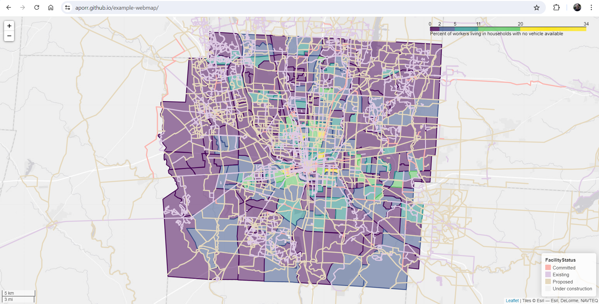
The screenshot above shows the webmap that is produced by this notebook. It includes two layers:
- Percent of workers living in households with no vehicle access by census tract
- Central Ohio bicycle infrastructure facilities by completion status
The completed webmap consists of a single HTML file that includes all of the required Javascript code (automatically generated) as well as all of the data that is displayed on the map. It includes typical user interface features such as pan/zoom, tooltips, and pop-ups.
Why would I want a standalone webmap?
- You can't afford to use a commercial service (such as ArcGIS Online).
- You need to share a restricted-access map with parties who cannot access a commercial service.
- You want to hand over the completed map so you aren't obligated to host it indefinitely.
- You want the map to include niche features that the commercial services don't support.
- You want to automate production of the map.
- You want to revision control the map (e.g. git).
- You want to embed the map in a custom web app more seamlessly
What are the steps?
- Set up the environment
- Prepare the data
- Prototype the webmap using Jupyter
- Export the webmap to a standalone HTML file
- Publish the HTML file on a webserver
Prerequisites
- Python 3.x
- GeoPandas library
- Jupyter (optional, but helpful for prototyping)
- GitHub acccount (optional, if you wish to publish using GitHub)
- Webserver (optional, if you wish to publish without GitHub)
- Basic familiarity with Python and GitHub
Demo of webmap creation and export
Environment setup
The following Python packages are required to execute this notebook. All required packages can be installed automatically using pip. See README.md for more details.
import pandas as pd # For manipulating tabular data
import geopandas as gpd # Extension of pandas for manipulating spatial data
import requests # For retrieving data from the Census API
import json # For transforming data from the Census API
import os # For manipulating files
Prepare the data
The webmap produced by this script consists of Central Ohio bicycle infrastructure line data overlaid on tract-level rates of zero-vehicle households from the American Community Survey. The bike infrastructure data includes proposed routes, therefore the webmap could potentially be used as a tool to prioritize construction of routes to serve areas with limited vehicle access.
Load tract geographies
The census tract geographies for Ohio are downloaded from the Census TIGER program as a zipped Shapefile, which is loaded directly into a GeoPandas GeoDataFrame.
tractsRaw = gpd.read_file("https://www2.census.gov/geo/tiger/TIGER2022/TRACT/tl_2022_39_tract.zip")
The geography dataset includes tracts for all of Ohio. Extract only the tracts for Franklin County (FIPS code 049) in Central Ohio. Extract only the geometries for the tracts; the other attributes are not needed. Use the unique Census identifier (GEOID) as the index (primary key). Reproject the data to the Ohio State Plane South coordinate reference system (EPSG:3735) to match the bike infrastucture data.
tracts = tractsRaw.loc[
(tractsRaw["STATEFP"] == '39') &
(tractsRaw["COUNTYFP"] == '049')
].copy() \
.filter(items=["GEOID","geometry"], axis="columns") \
.set_index("GEOID") \
.to_crs("epsg:3735")
Show a selection of the data.
tracts.head()
| geometry | |
|---|---|
| GEOID | |
| 39049006392 | POLYGON ((1812678.02 769514.607, 1812796.958 7... |
| 39049006500 | POLYGON ((1805161.518 730017.428, 1805222.134 ... |
| 39049006600 | POLYGON ((1806233.249 728073.229, 1806465.314 ... |
| 39049006710 | POLYGON ((1822275.804 759052.354, 1822275.413 ... |
| 39049006721 | POLYGON ((1818673.74 766164.975, 1818684.28 76... |
Show a basic map of the tract geographies.
tracts.plot(figsize=(10,10))
<Axes: >

Load means of transportation by Census tract
The tract-level vehicle access data (and some other variables) are downloaded from the Census ACS 2022 5-Year Estimates API using a custom HTTP GET request. The data is provided as a list of records in JSON format. The first record (list item zero) represents the column headers, so this is extracted first. The remaining records are loaded into a Pandas DataFrame.
The URL and query parameters used for the API request could have been constructed manually using the instructions at the link above, however in this case they were obtained using the new "API" feature available in the data.census.gov tool, as shown in the screenshot below. The query fetches all variables available in Table B08141 for all tracts in Franklin County.
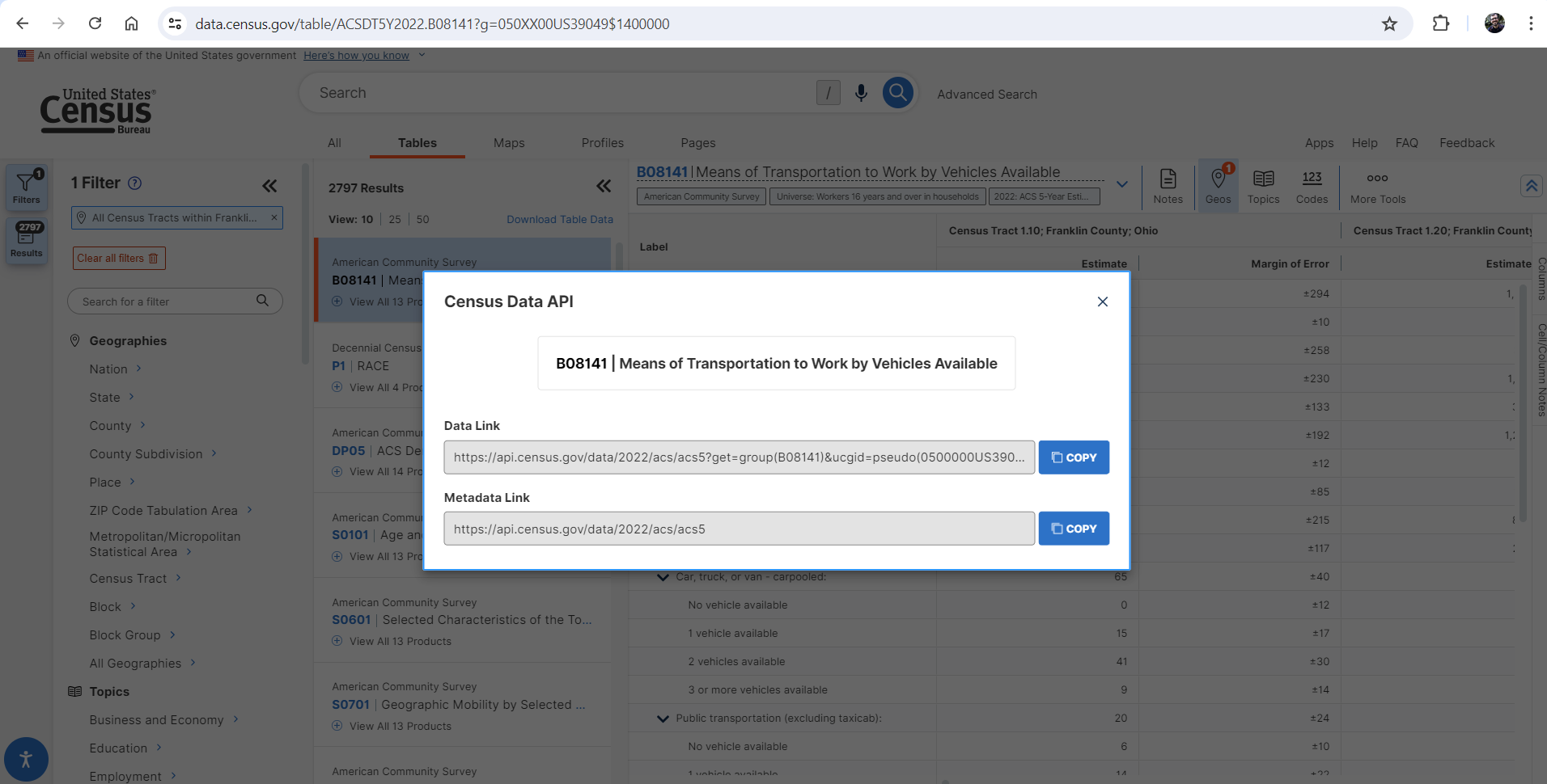
Send the request, extract the column headers, and create the DataFrame.
r = requests.get("https://api.census.gov/data/2022/acs/acs5?get=group(B08141)&ucgid=pseudo(0500000US39049$1400000)")
headers = r.json()[0]
commuteRaw = pd.DataFrame.from_records(r.json()[1:], columns=headers)
Create a working copy of the data and create a shortened version of the geographic identifiers to match the identifiers used in the TIGER data.
commute = commuteRaw.copy()
commute["GEOID"] = commute["GEO_ID"].apply(lambda x:x.split("US")[1])
Create a list of the variables to include in the webmap, and create human-readable aliases for them.
commuteVars = {
"B08141_001E":"Workers 16 and over in households",
"B08141_002E":"No vehicles available",
"B08141_003E":"1 vehicle available",
"B08141_004E":"2 vehicles available",
"B08141_005E":"3 vehicles available",
"B08141_006E":"Drove alone",
"B08141_011E":"Carpooled",
"B08141_016E":"Public transportation",
"B08141_021E":"Walked",
"B08141_026E":"Commute by other means",
"B08141_035E":"Worked from home"
}
Use the GEOID as the index (primary key). Extract only the required variables and rename them as indicated above. Make sure all variables are cast as integers. Finally, compute the percentage of workers 16 and over in households which live in a household with no vehicles available.
commute = commute \
.set_index("GEOID") \
.filter(items=commuteVars.keys(), axis="columns") \
.rename(columns=commuteVars) \
.astype("int")
commute["No vehicles available (%)"] = commute["No vehicles available"].div(commute["Workers 16 and over in households"], fill_value=0).mul(100, fill_value=0)
Show a selection of the data.
commute.head()
| Workers 16 and over in households | No vehicles available | 1 vehicle available | 2 vehicles available | 3 vehicles available | Drove alone | Carpooled | Public transportation | Walked | Commute by other means | Worked from home | No vehicles available (%) | |
|---|---|---|---|---|---|---|---|---|---|---|---|---|
| GEOID | ||||||||||||
| 39049000110 | 2273 | 6 | 580 | 1326 | 361 | 1516 | 65 | 20 | 15 | 198 | 81 | 0.263968 |
| 39049000120 | 1981 | 99 | 331 | 1152 | 399 | 1266 | 19 | 18 | 21 | 10 | 114 | 4.997476 |
| 39049000210 | 2029 | 122 | 538 | 883 | 486 | 1160 | 120 | 116 | 59 | 53 | 70 | 6.012814 |
| 39049000220 | 2293 | 0 | 455 | 1483 | 355 | 1420 | 201 | 50 | 17 | 103 | 63 | 0.000000 |
| 39049000310 | 1452 | 9 | 377 | 727 | 339 | 1067 | 159 | 7 | 0 | 16 | 26 | 0.619835 |
Load Central Ohio bikeways
MORPC maintains a spatial dataset describing bicycle infrastructure in Central Ohio. The dataset includes the status of each facility, including existing, proposed, committed/funded, and under construction. A public version of the dataset is hosted in MORPC's ArcGIS Online instance. The data is available via the built-in ArcGIS REST API, however queries are limited to 2000 records. The entire dataset consists of 8000+ records, therefore it is necessary to download all of the records using a series of queries. The following block queries the API to determine the total record count, then iteratively requests the records in 2000-record chunks until all records have been downloaded. The data is provided in GeoJSON format, therefore it can be loaded directly into a GeoPandas GeoDataFrame. The chunks are concatenated (appended) to create a dataframe consisting of the entire collection of records.
# Request the total record count from the API
r = requests.get("https://services1.arcgis.com/EjjnBtwS9ivTGI8x/arcgis/rest/services/Bikeways_CentralOhio/FeatureServer/1/query?outFields=*&where=1%3D1&returnCountOnly=true&f=json")
# Extract the JSON from the API response
result = r.json()
# Extract the total record count from the JSON
totalRecordCount = result["count"]
firstTime = True
offset = 0
exceededLimit = True
recordCount = 2000
while offset < totalRecordCount:
print("Downloading records {} to {}".format(offset+1, offset + recordCount))
# Request 2000 records from the API starting with the record indicated by offset.
# Configure the request to include only the required fields, to project the geometries to
# Ohio State Plane South coordinate reference system (EPSG:3735), and to format the data as GeoJSON
r = requests.get("https://services1.arcgis.com/EjjnBtwS9ivTGI8x/arcgis/rest/services/Bikeways_CentralOhio/FeatureServer/1/query?outFields=OBJECTID,FacilityStatus,FacilityType&where=1%3D1&f=geojson&outSR=3735&resultOffset={}&resultRecordCount={}".format(offset, recordCount))
# Extract the GeoJSON from the API response
result = r.json()
# Read this chunk of data into a GeoDataFrame
temp = gpd.GeoDataFrame.from_features(result["features"], crs="epsg:3735")
if firstTime:
# If this is the first chunk of data, create a permanent copy of the GeoDataFrame that we can append to
trailsRaw = temp.copy()
firstTime = False
else:
# If this is not the first chunk, append to the permanent GeoDataFrame
trailsRaw = pd.concat([trailsRaw, temp], axis="index")
# Increase the offset so that the next request fetches the next chunk of data
offset += 2000
print("All records downloaded")
Downloading records 1 to 2000 Downloading records 2001 to 4000 Downloading records 4001 to 6000 Downloading records 6001 to 8000 Downloading records 8001 to 10000 All records downloaded
Remove facilties that no longer exist (i.e. where status is "removed"). Convert the codes for facility status and facility type to human-readable text.
trails = trailsRaw.loc[trailsRaw["FacilityStatus"] != "REM"].copy() \
.filter(items=["FacilityStatus","FacilityType","geometry"])
trails["FacilityStatus"] = trails["FacilityStatus"].map({
"EX":"Existing",
"COM":"Committed",
"PRO":"Proposed",
"UND":"Under construction"
})
trails["FacilityType"] = trails["FacilityType"].map({
'PS': 'Paved Shoulder',
'RT': 'Signed Bicycle Route',
'SH': 'Shared Lane Markings',
'BB': 'Bicycle Boulevard',
'MBT': 'Mountain Bike Trail',
'STR': 'Street Crossing',
'PC': 'Pedestrian Connector',
'PATH': 'Multi-use Path',
'PT': 'Pedestrian Trail',
'PRO': 'Proposed',
'COM': 'Committed',
'NONE': 'No Connection',
'LANE': 'Bicycle Lane',
'PBL': 'Protected Bicycle Lane'
})
Show a selection of the data.
trails.head()
| FacilityStatus | FacilityType | geometry | |
|---|---|---|---|
| 0 | Proposed | Proposed | LINESTRING (1815340.339 887243.451, 1815290.44... |
| 1 | Proposed | Proposed | LINESTRING (1803621.977 887185.603, 1803652.13... |
| 2 | Proposed | Proposed | LINESTRING (1813076.868 887400.211, 1812935.86... |
| 3 | Proposed | Proposed | LINESTRING (1802465.467 886678.783, 1803540.35... |
| 4 | Proposed | Proposed | LINESTRING (1784373.787 886500.139, 1783966.76... |
Plot the bike infrastructure overlaid on the census tracts to get a sense of its spatial extent and patterns.
ax = tracts.plot(color="gray", figsize=(15,15))
trails.plot(ax=ax, column="FacilityStatus", legend=True)
<Axes: >

Join means of transportation to tract geographies
Currently we have a spatial dataset that includes only the census tract geographies and a separate table that includes commute-related census variables. To see the spatial patterns in the commuting data, we need to combine the two datasets. Join the table to the geographies, aligning on the unique identifiers (GEOID).
tractsEnriched = tracts.join(commute)
Show a selection of the combined data.
tractsEnriched.head()
| geometry | Workers 16 and over in households | No vehicles available | 1 vehicle available | 2 vehicles available | 3 vehicles available | Drove alone | Carpooled | Public transportation | Walked | Commute by other means | Worked from home | No vehicles available (%) | |
|---|---|---|---|---|---|---|---|---|---|---|---|---|---|
| GEOID | |||||||||||||
| 39049006392 | POLYGON ((1812678.02 769514.607, 1812796.958 7... | 2052 | 0 | 137 | 1208 | 707 | 1398 | 62 | 14 | 0 | 51 | 92 | 0.000000 |
| 39049006500 | POLYGON ((1805161.518 730017.428, 1805222.134 ... | 1597 | 4 | 225 | 1070 | 298 | 1125 | 64 | 0 | 11 | 0 | 85 | 0.250470 |
| 39049006600 | POLYGON ((1806233.249 728073.229, 1806465.314 ... | 2097 | 0 | 130 | 1311 | 656 | 1431 | 96 | 10 | 51 | 33 | 103 | 0.000000 |
| 39049006710 | POLYGON ((1822275.804 759052.354, 1822275.413 ... | 1469 | 16 | 312 | 853 | 288 | 1186 | 107 | 0 | 42 | 0 | 48 | 1.089176 |
| 39049006721 | POLYGON ((1818673.74 766164.975, 1818684.28 76... | 1893 | 0 | 185 | 1241 | 467 | 1482 | 44 | 0 | 54 | 21 | 40 | 0.000000 |
Plot the census tracts, symbolizing them by percentage of workers age 16 and over who live in households with no vehicles available to get a sense of the spatial patterns of vehicle access.
tractsEnriched.plot(column="No vehicles available (%)", cmap="viridis", legend=True, figsize=(10,10))
<Axes: >

Prototype the webmap
Cartography is part art and part science, and GeoPandas allows for a significant degree of customization, therefore some prototyping is typically warranted to produce the most effective webmap possible. Three attempts are captured in the following subsections:
- The first attempt produces a webmap that is largely unconfigured. That is, it relies on the default configuration established by GeoPandas.
- The second attempt applies some custom styling to the symbols used for the tract-level vehicle access data and the bike infrastructure.
- The third attempt uses percent of workers with no vehicle access instead of the raw estimates and classifies the percentages into five classes using the Fisher-Jenks method. A cleaner basemap is used, as well as (arguably) more legible symbols for the layers. Several user interface elements are also customized, including the default zoom level, and more intentional use of popups and mouseover interactions.
First attempt (minimally configured)
map1 = tractsEnriched.explore(column="No vehicles available")
trails.explore(m=map1, column="FacilityStatus")
Second attempt (better configured)
map2 = tractsEnriched.explore(
column="No vehicles available",
cmap="summer",
style_kwds={
"fillOpacity":1
}
)
trails.explore(m=map2,
column="FacilityStatus",
cmap="Paired",
style_kwds={
"weight":2,
}
)
Final attempt (fully configured)
map3 = tractsEnriched.explore(
column="No vehicles available (%)",
scheme="FisherJenks",
k=5,
tiles="Esri.WorldGrayCanvas",
cmap="viridis",
tooltip=False,
popup=commuteVars.values(),
highlight=False,
zoom_start=11,
legend_kwds={
"caption": "Percent of workers living in households with no vehicle available"
}
)
trails.explore(m=map3,
column="FacilityStatus",
cmap="Pastel1",
style_kwds={"weight":3},
tooltip=True
)
Export the webmap
After the map is configured how we like it, we can save it as a standalone HTML file. Note that this file includes the entire webmap application and all of the data displayed on the map. Depending on how much data is included, the file may take up a significant amount of space on disk and it may require a large amount of memory to display it in the web browser. This method, while convenient for some applications, is not a substitute for GIS software or a more full-featured webmap service.
map3.save("webmap.html")
Demo of publishing using GitHub Pages
The following subsections will walk you through the process of creating a GitHub repository for your webmap, uploading the standalone HTML file to the repository, and setting up GitHub Pages to make the webmap available to the public. The instructions and screenshots assume that the process is carried out using the GitHub website, however most steps could also be accomplished using the git command line utility or the GitHub Desktop app.
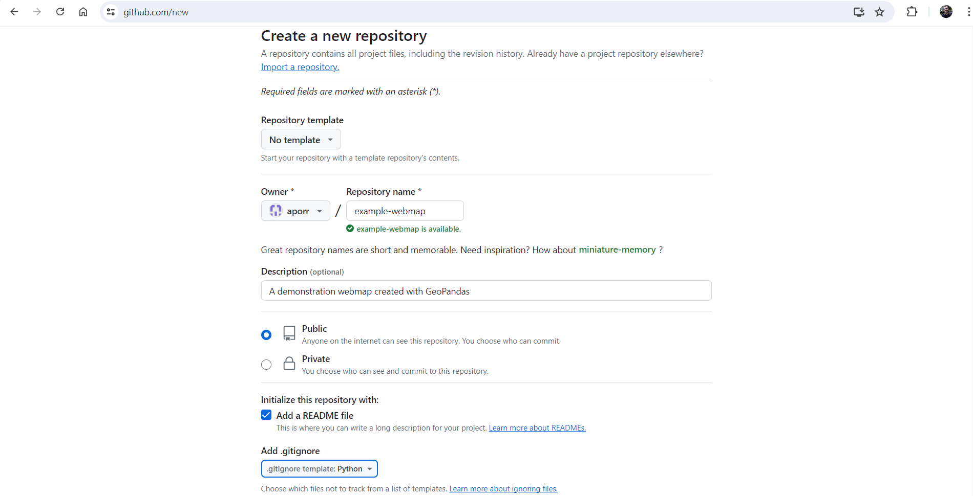
Create a git repository
Upload the webmap HTML file to the repository
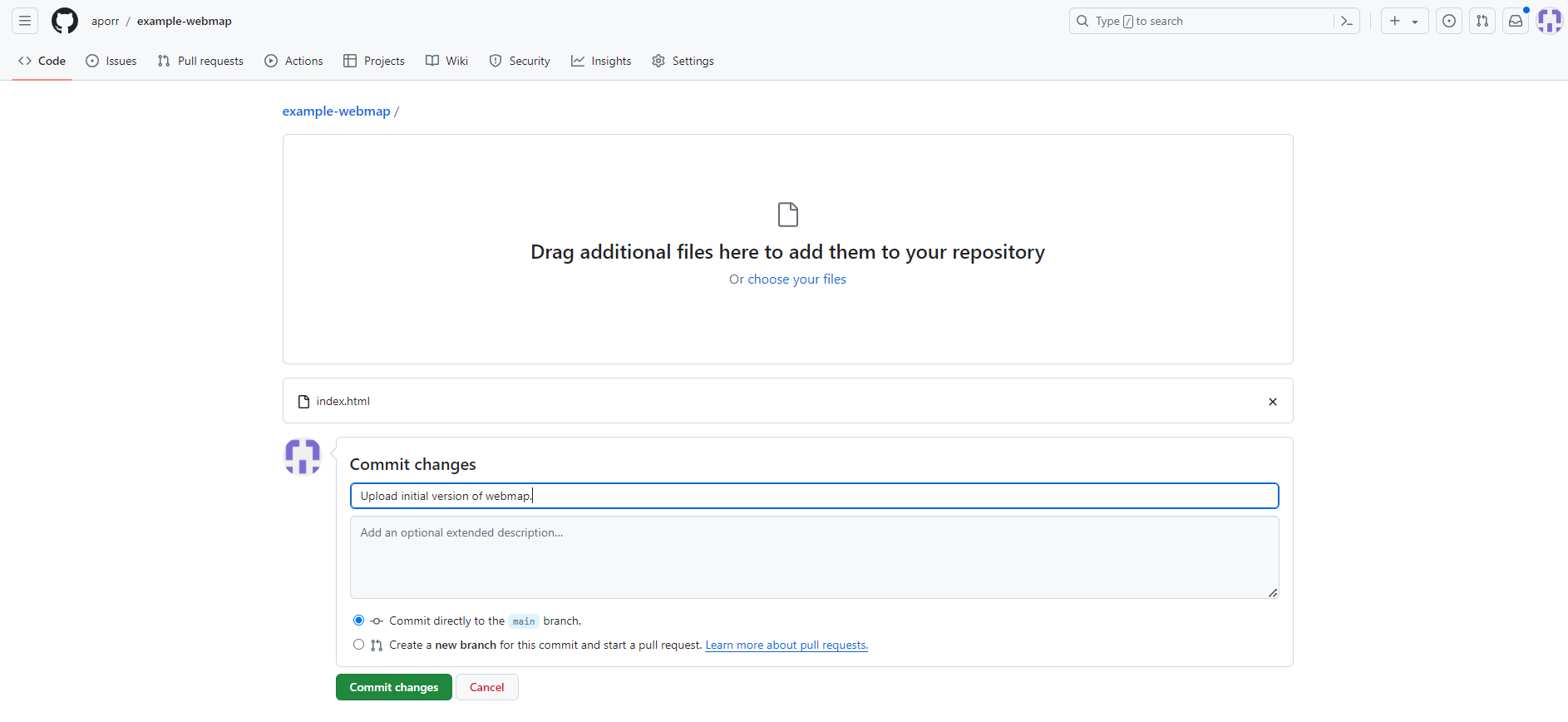
Notes:
- The file MUST be in the repository root or in a directory called "docs".
- The file SHOULD be called "index.html".
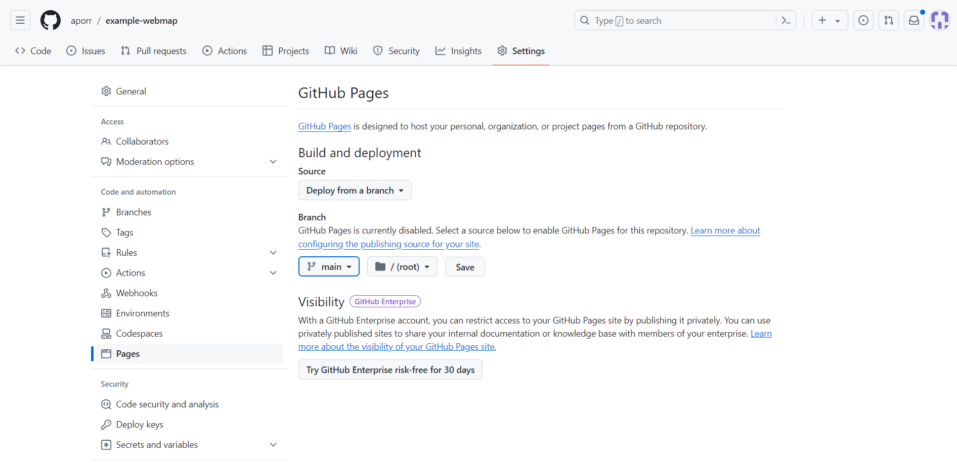
Enable GitHub Pages for the repository
Access the webmap
Notes:
- The URL will have the format:
http://username.github.io/repository_name - If you didn't call the file
index.html, you'll have to specify the file name like this:http://username.github.io/repository_name/filename.html - It may take a few minutes after enabling GitHub Pages or pushing a new version for the content to be available.